# 综合医学分析项目 {#sec-comprehensive}
```{r}
#| label: check-packages
#| message: false
# 设置CRAN镜像为中国合肥镜像
options(repos = c(CRAN = "https://mirrors.ustc.edu.cn/CRAN/"))

# 检查并安装所需的R包
required_packages <- c(
  "tidyverse",     # 数据处理和可视化
  "caret",         # 机器学习
  "pROC",          # ROC曲线分析
  "rms",           # 回归建模
  "medicaldata",   # 医学数据集
  "tidymodels",    # 建模框架
  "MatchIt",       # 倾向评分匹配
  "sf",            # 空间数据处理
  "tmap"           # 专题地图
)

# 检查并安装缺失的包
new_packages <- required_packages[!(required_packages %in% installed.packages()[,"Package"])]
if(length(new_packages)) install.packages(new_packages, dependencies = TRUE)

# 加载所有包
invisible(lapply(required_packages, library, character.only = TRUE))
```
## 临床预测模型开发 {#sec-prediction-model}
### 特征工程处理 {#sec-feature-engineering}
```{r}
#| label: setup
#| message: false
library(tidyverse)
library(caret)
library(pROC)
library(rms)
library(tidymodels)

# 创建模拟临床数据
set.seed(123)
n_patients <- 500

# 生成模拟数据
clinical_data <- tibble(
  age = rnorm(n_patients, mean = 50, sd = 15),
  weight = rnorm(n_patients, mean = 70, sd = 15),
  height = rnorm(n_patients, mean = 170, sd = 10),
  asa = sample(1:4, n_patients, replace = TRUE),
  mallampati = sample(1:4, n_patients, replace = TRUE)
)

# 特征工程
model_data <- clinical_data %>%
  # 创建新特征
  mutate(
    bmi = weight / ((height/100)^2),
    age_group = cut(age, breaks = c(0, 40, 60, 100),
                   labels = c("青年", "中年", "老年")),
    risk_score = case_when(
      asa < 3 & bmi < 30 ~ "低风险",
      asa >= 4 | bmi >= 35 ~ "高风险",
      TRUE ~ "中等风险"
    ),
    # 模拟困难插管的概率
    difficult_intubation = rbinom(n_patients, 1,
      plogis(-3 + 0.03*age + 0.1*bmi + 0.5*asa + 0.7*mallampati))
  )

# 划分训练集和测试集
set.seed(123)
train_index <- createDataPartition(model_data$difficult_intubation, p = 0.7, list = FALSE)
train_data <- model_data[train_index, ]
test_data <- model_data[-train_index, ]
```
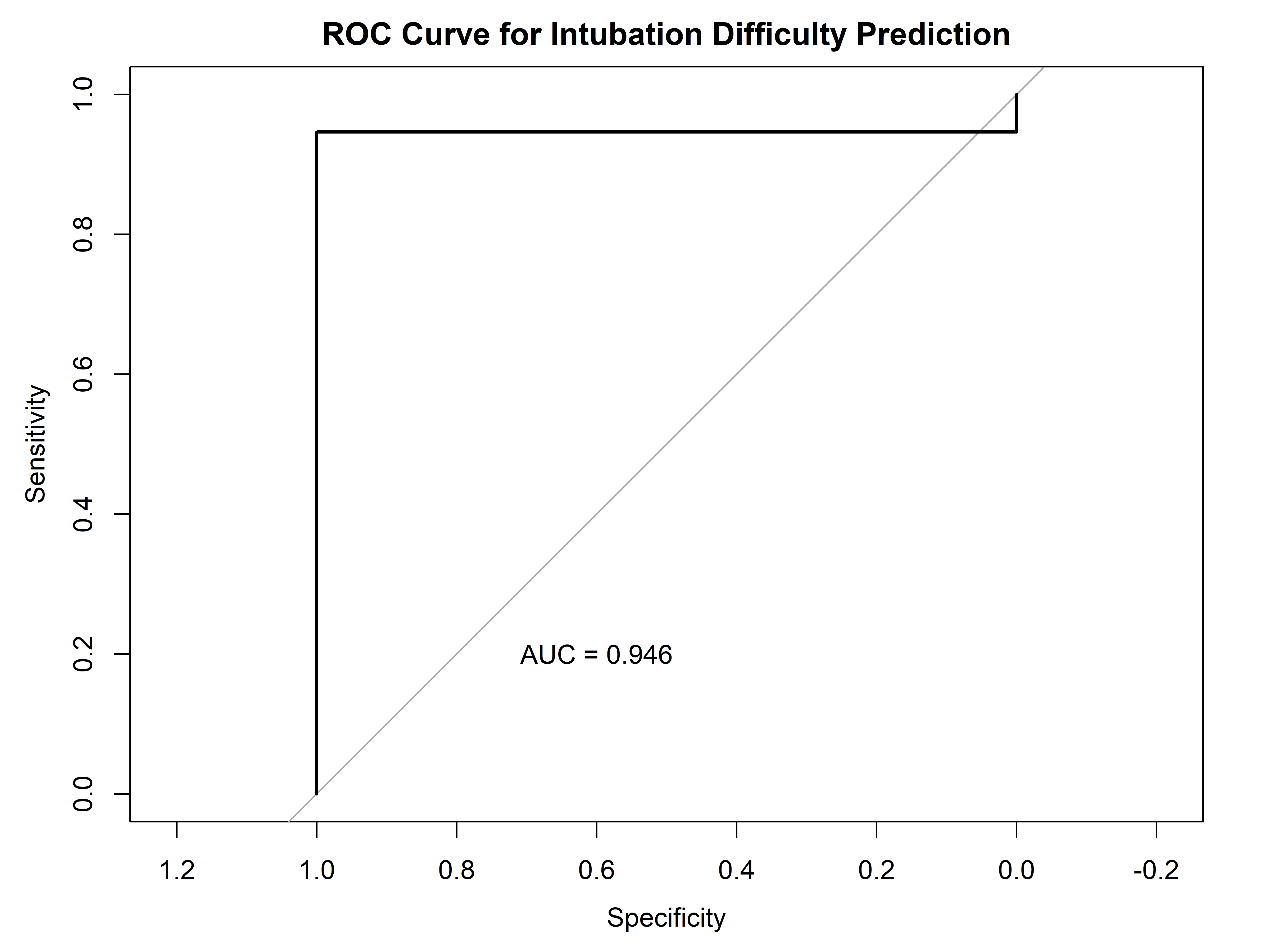
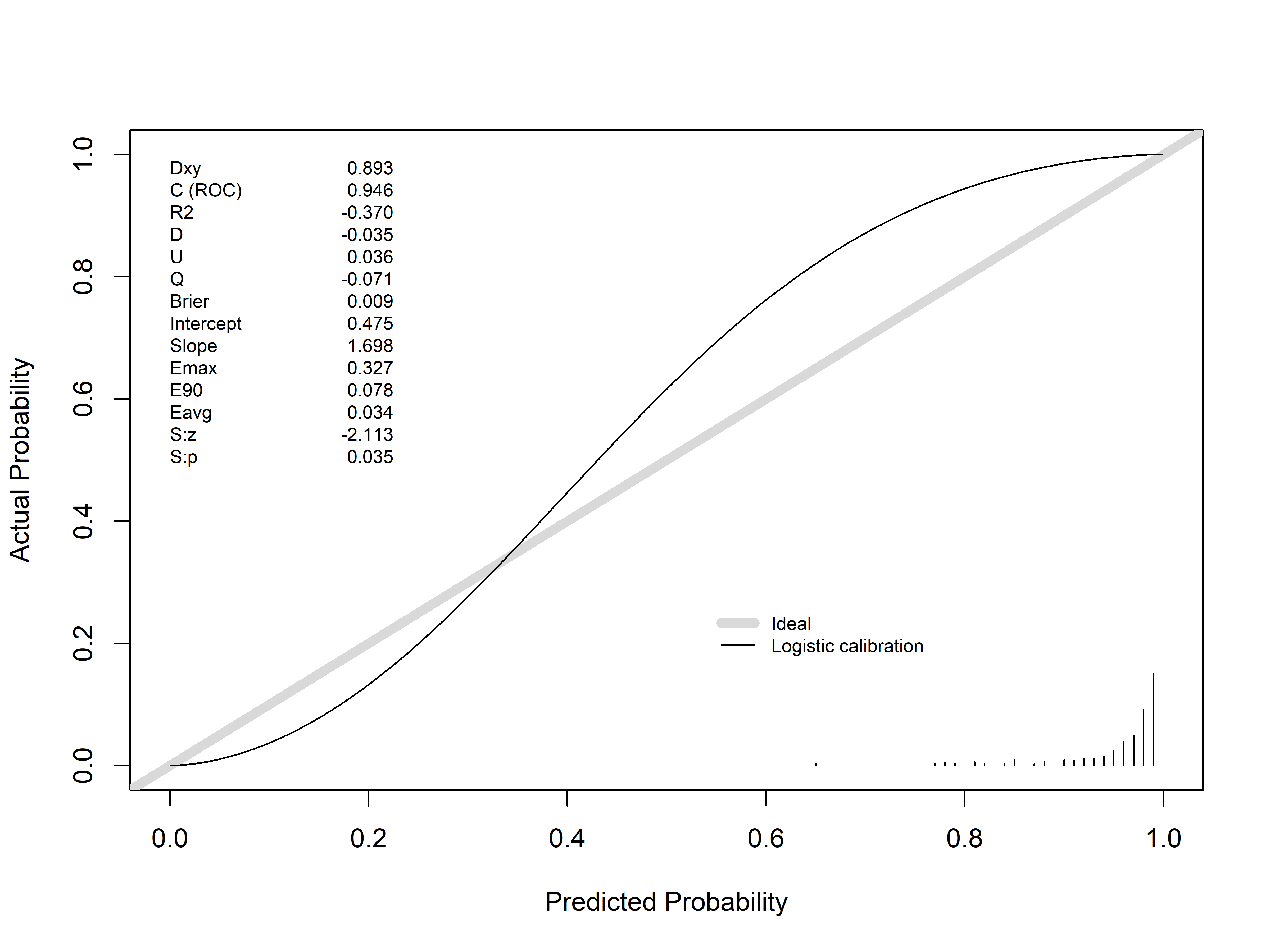
### 模型验证与校准 {#sec-model-validation}
```{r}
#| label: model-validation
# 构建logistic回归模型
model <- glm(difficult_intubation ~ age + bmi + asa + mallampati,
            family = binomial,
            data = train_data)

# 模型性能评估
predictions <- predict(model, newdata = test_data, type = "response")
roc_curve <- roc(test_data$difficult_intubation, predictions)

# 绘制ROC曲线
plot(roc_curve, main = "ROC Curve for Intubation Difficulty Prediction")
auc <- auc(roc_curve)
text(0.6, 0.2, paste("AUC =", round(auc, 3)))
# 校准曲线
val.prob(predictions, test_data$difficult_intubation, smooth = FALSE)
```
## 真实世界研究分析 {#sec-real-world}
### 电子病历数据挖掘 {#sec-ehr-mining}
```{r}
#| label: ehr-analysis
# 模拟电子病历数据
set.seed(123)
n_patients <- 1000
ehr_data <- tibble(
patient_id = 1:n_patients,
age = rnorm(n_patients, 55, 15),
gender = sample(c("男", "女"), n_patients, replace = TRUE),
diagnosis = sample(c("高血压", "糖尿病", "冠心病", "正常"),
n_patients, replace = TRUE, prob = c(0.3, 0.2, 0.1, 0.4)),
medication = sample(c("药物A", "药物B", "药物C", "无"),
n_patients, replace = TRUE),
visits = rpois(n_patients, 3),
cost = rlnorm(n_patients, 8, 1)
)
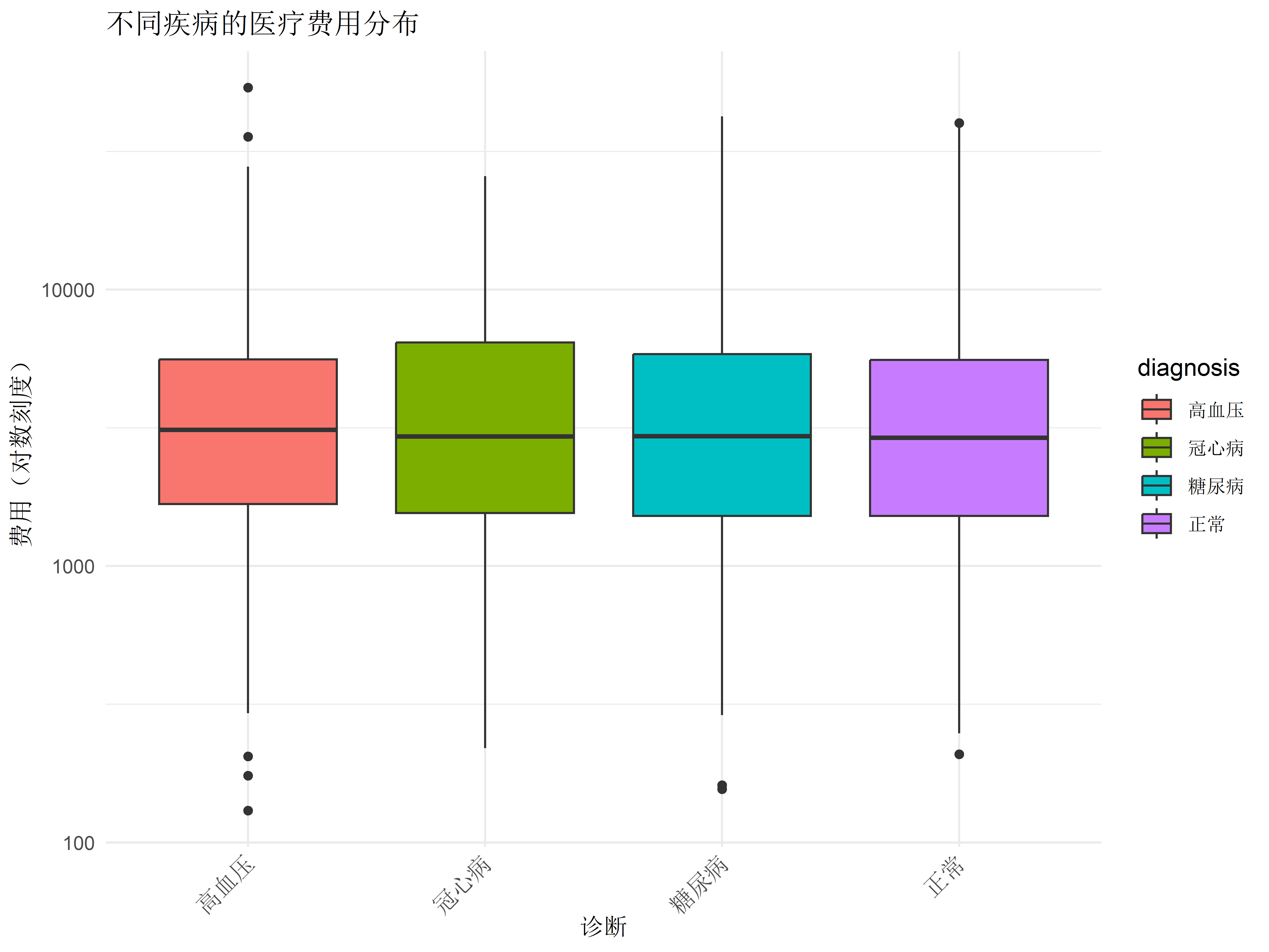
# 描述性分析
ehr_summary <- ehr_data %>%
group_by(diagnosis) %>%
summarise(
患者数 = n(),
平均年龄 = mean(age),
平均就诊次数 = mean(visits),
平均费用 = mean(cost)
)
# 可视化分析
ggplot(ehr_data, aes(x = diagnosis, y = cost, fill = diagnosis)) +
geom_boxplot() +
scale_y_log10() +
labs(title = "不同疾病的医疗费用分布",
x = "诊断",
y = "费用(对数刻度)") +
theme_minimal() +
theme(axis.text.x = element_text(angle = 45, hjust = 1))
```
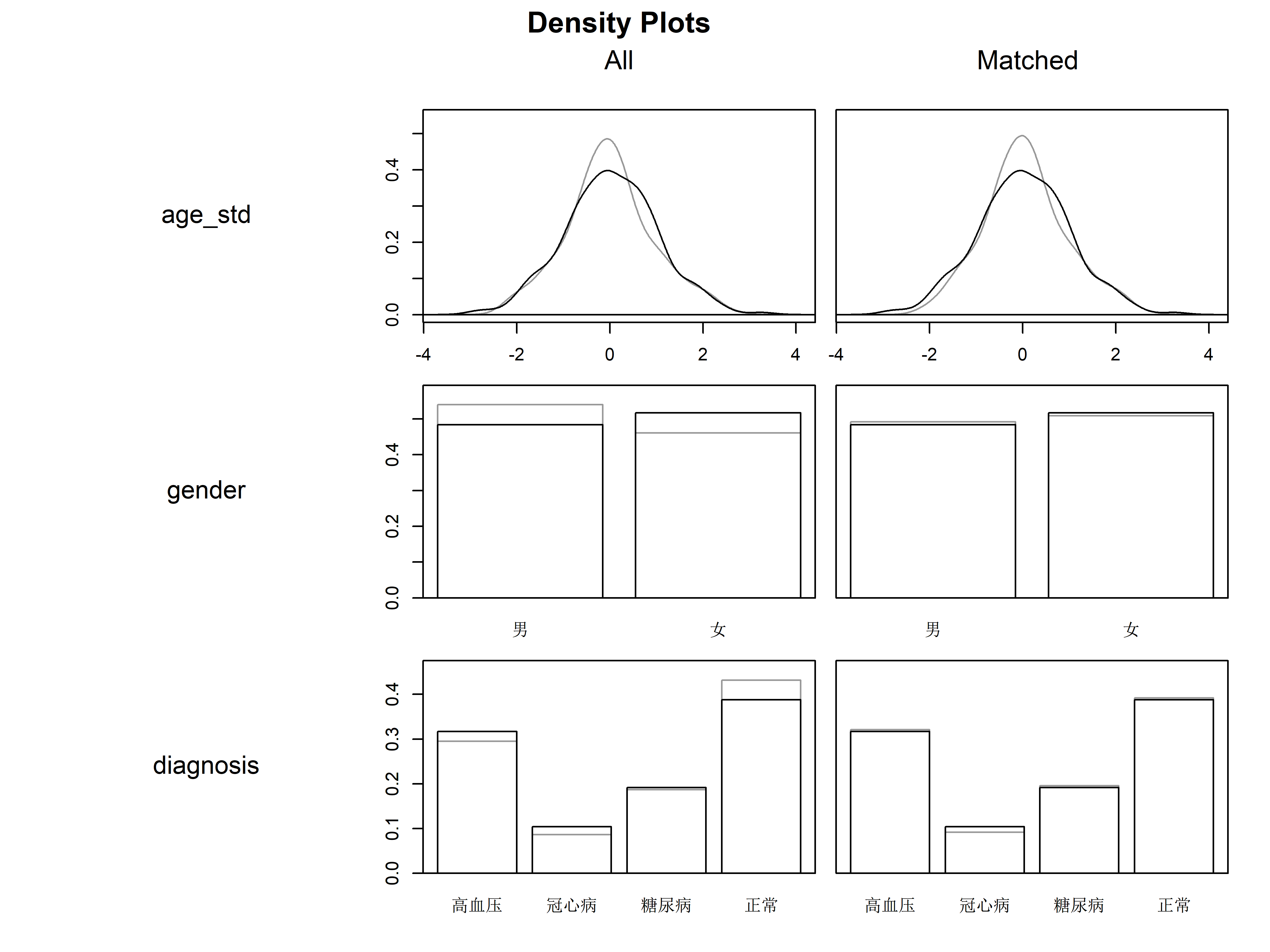
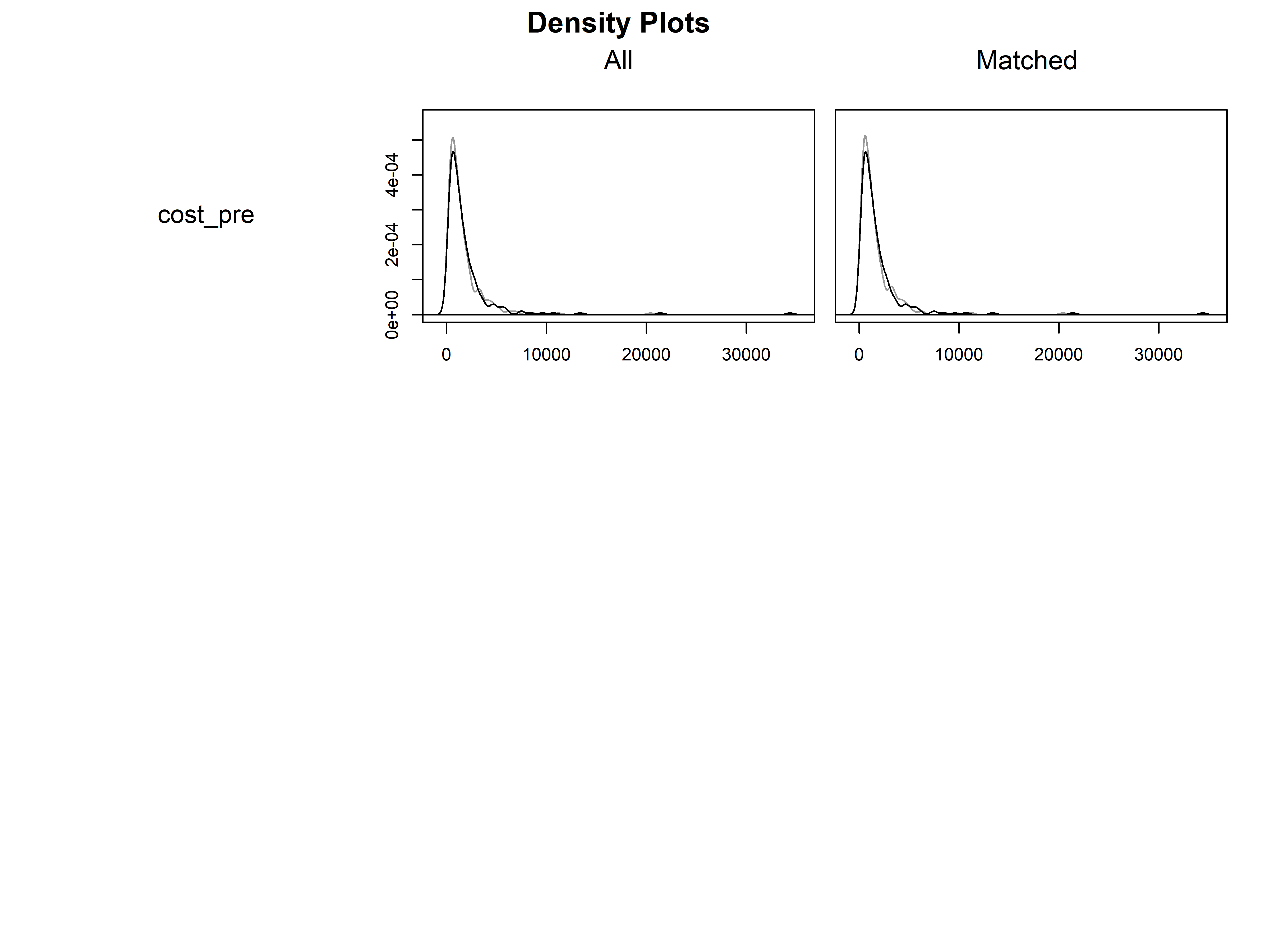
### 倾向评分匹配(PSM) {#sec-psm}
```{r}
#| label: psm-analysis
library(MatchIt)

# 准备数据进行PSM
treatment_data <- ehr_data %>%
  mutate(
    treatment = ifelse(medication == "药物A", 1, 0),
    age_std = scale(age),
    cost_pre = rlnorm(n_patients, 7, 1)
  ) %>%
  filter(medication %in% c("药物A", "药物B"))

# 进行PSM
m.out <- matchit(treatment ~ age_std + gender + diagnosis + cost_pre,
                data = treatment_data,
                method = "nearest",
                ratio = 1)

# 查看匹配结果
summary(m.out)
# 提取匹配后的数据
matched_data <- match.data(m.out)

# 评估平衡性
plot(m.out, type = "density", interactive = FALSE)
```
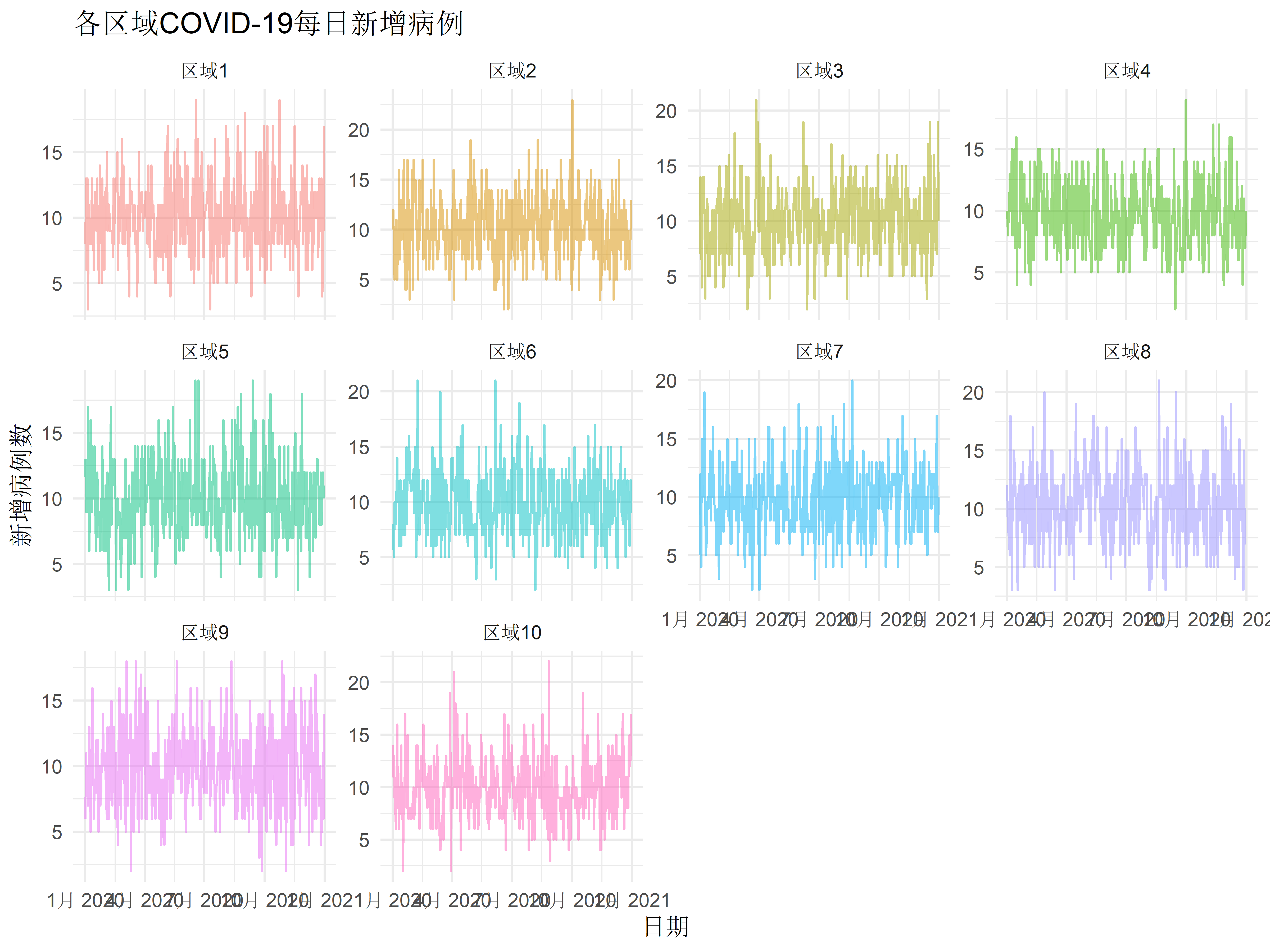
## COVID-19数据分析 {#sec-covid}
### 疫情时空分布分析 {#sec-spatiotemporal}
```{r}
#| label: covid-analysis
library(sf)
library(tmap)

# 模拟COVID-19疫情数据
dates <- seq(as.Date("2020-01-01"), as.Date("2020-12-31"), by = "day")
regions <- paste0("区域", 1:10)

covid_data <- expand.grid(
  date = dates,
  region = regions
) %>%
  mutate(
    cases = rpois(n(), lambda = 10),
    cumulative_cases = ave(cases, region, FUN = cumsum)
  )

# 时间趋势分析
ggplot(covid_data, aes(x = date, y = cases, color = region)) +
  geom_line(alpha = 0.5) +
  facet_wrap(~region, scales = "free_y") +
  labs(title = "各区域COVID-19每日新增病例",
       x = "日期",
       y = "新增病例数") +
  theme_minimal() +
  theme(legend.position = "none")
```
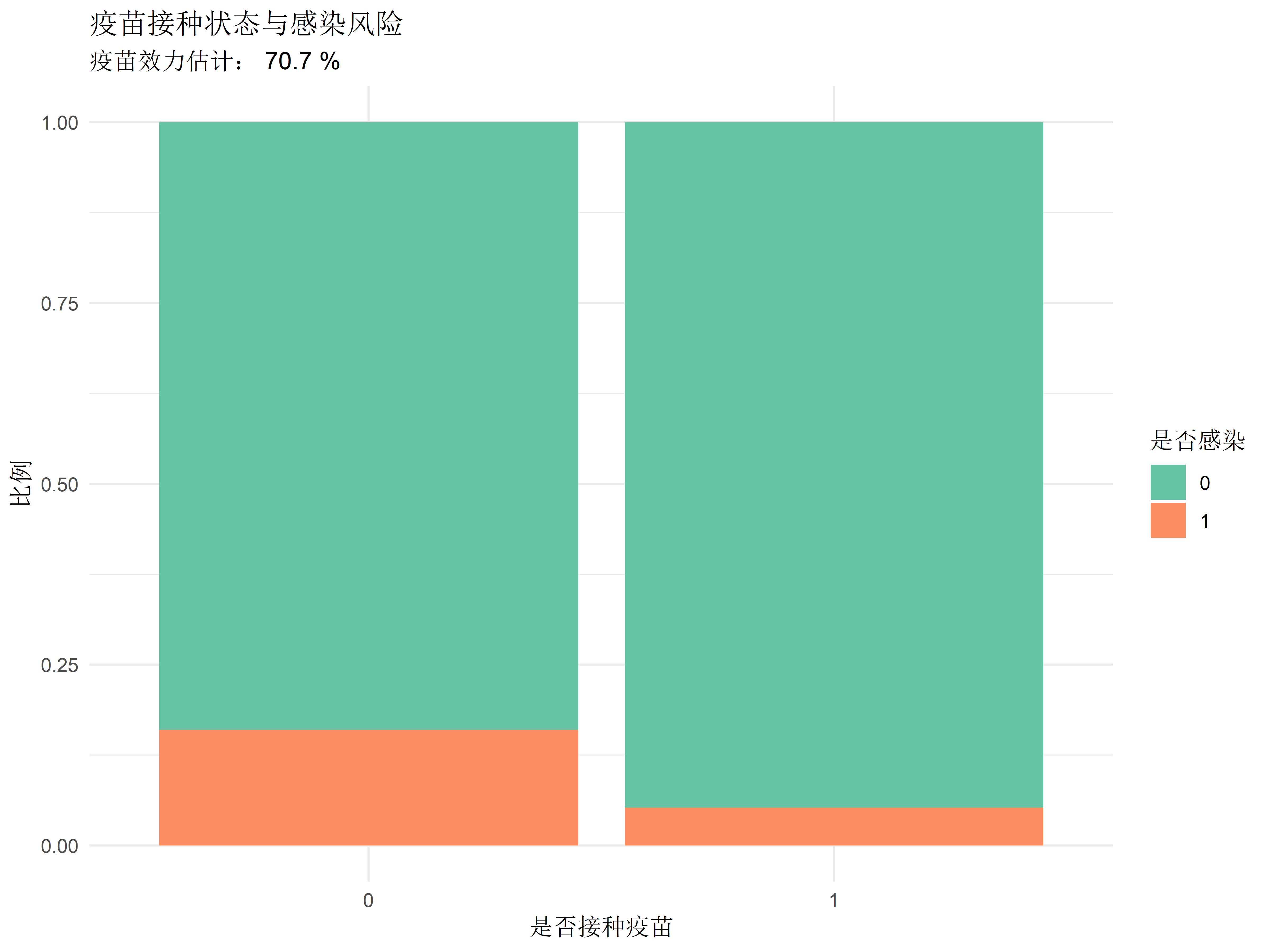
### 疫苗效果评估模型 {#sec-vaccine-effectiveness}
```{r}
#| label: vaccine-analysis
# 模拟疫苗接种数据
n_subjects <- 1000
vaccine_data <- tibble(
  subject_id = 1:n_subjects,
  age = rnorm(n_subjects, 45, 15),
  vaccinated = rbinom(n_subjects, 1, 0.7),
  risk_factor = rbinom(n_subjects, 1, 0.3),
  infected = rbinom(n_subjects, 1,
                   ifelse(vaccinated == 1, 0.05, 0.15))
)

# 分析疫苗效果
vaccine_model <- glm(infected ~ vaccinated + age + risk_factor,
                    family = binomial,
                    data = vaccine_data)

# 计算疫苗效果
ve <- (1 - exp(coef(vaccine_model)["vaccinated"])) * 100

# 可视化结果
ggplot(vaccine_data, aes(x = factor(vaccinated), fill = factor(infected))) +
  geom_bar(position = "fill") +
  labs(title = "疫苗接种状态与感染风险",
       subtitle = paste("疫苗效力估计:", round(ve, 1), "%"),
       x = "是否接种疫苗",
       y = "比例",
       fill = "是否感染") +
  scale_fill_brewer(palette = "Set2") +
  theme_minimal()
```
::: {.callout-tip}
## 练习
1. 使用自己的数据开发预测模型
2. 进行真实世界研究数据分析
3. 评估医疗干预的效果
4. 进行时空数据可视化
:::
## 本章小结
在本章中,我们学习了:
1. 如何开发和验证临床预测模型
2. 真实世界研究数据的分析方法
3. 倾向评分匹配的应用
4. 疫情数据的时空分析技术
::: {.callout-important}
## 持续学习
感谢您阅读本书!如需获取更多医学统计分析资源、代码更新和案例分享,欢迎关注微信公众号【R语言与可视化】。
您还可以:
- 在公众号后台留言交流学习心得
- 获取本书示例代码的完整版本
- 了解最新的R语言医学应用动态
:::