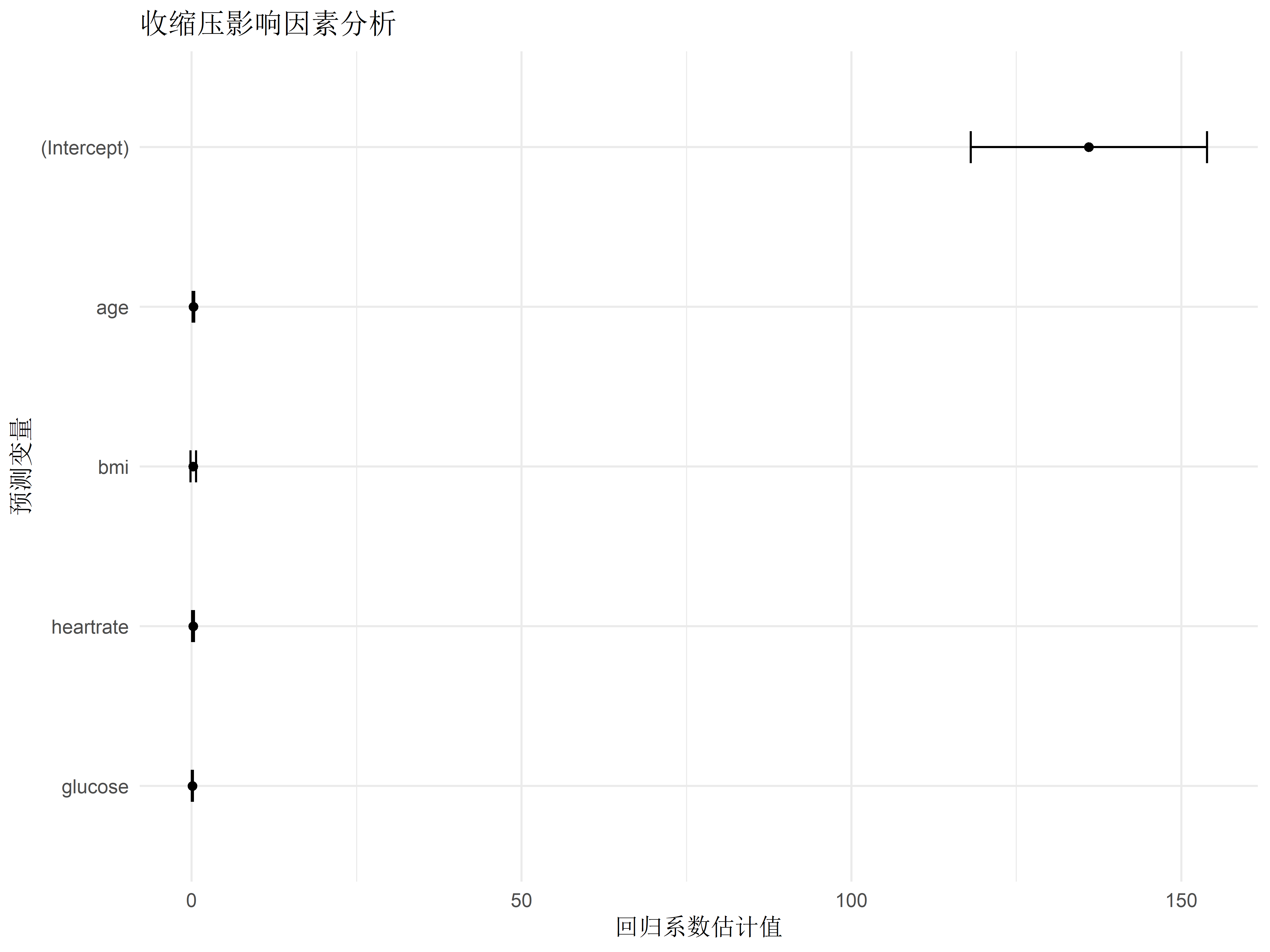
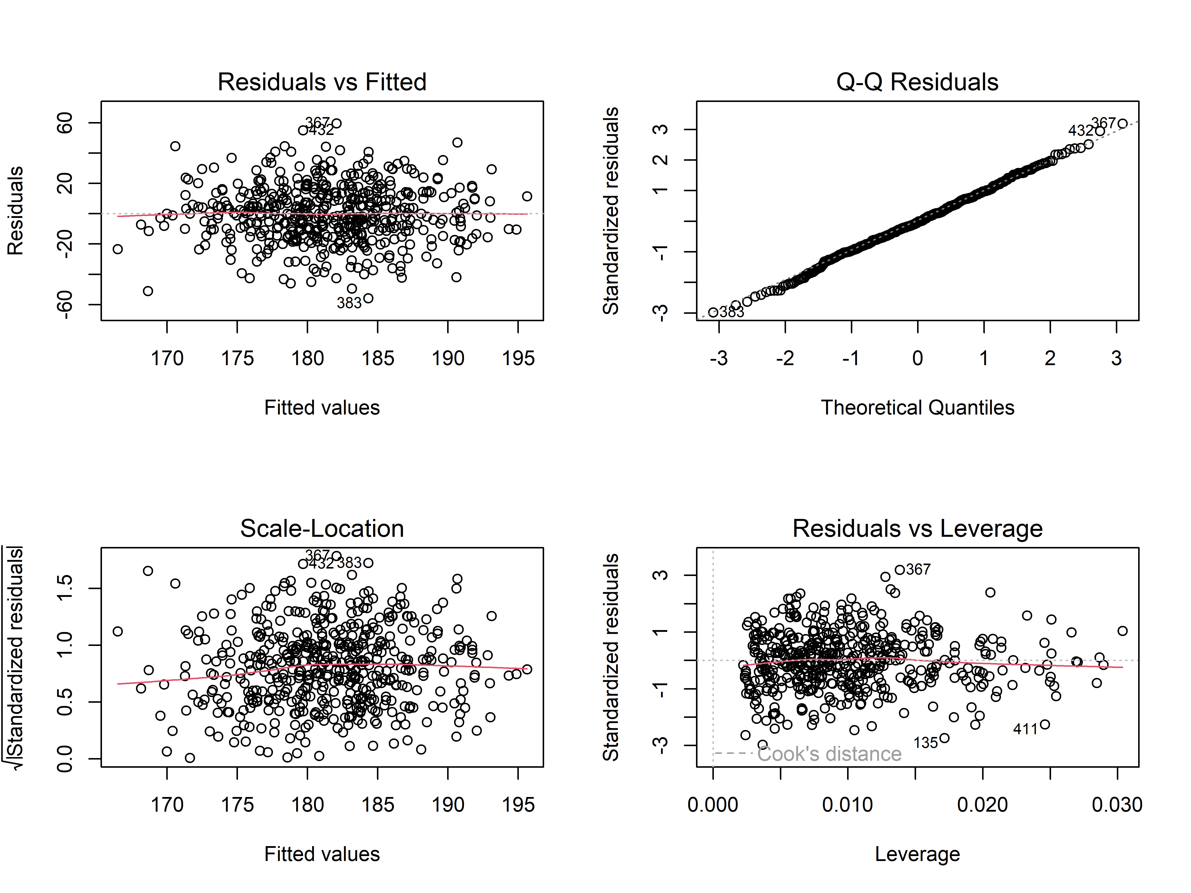
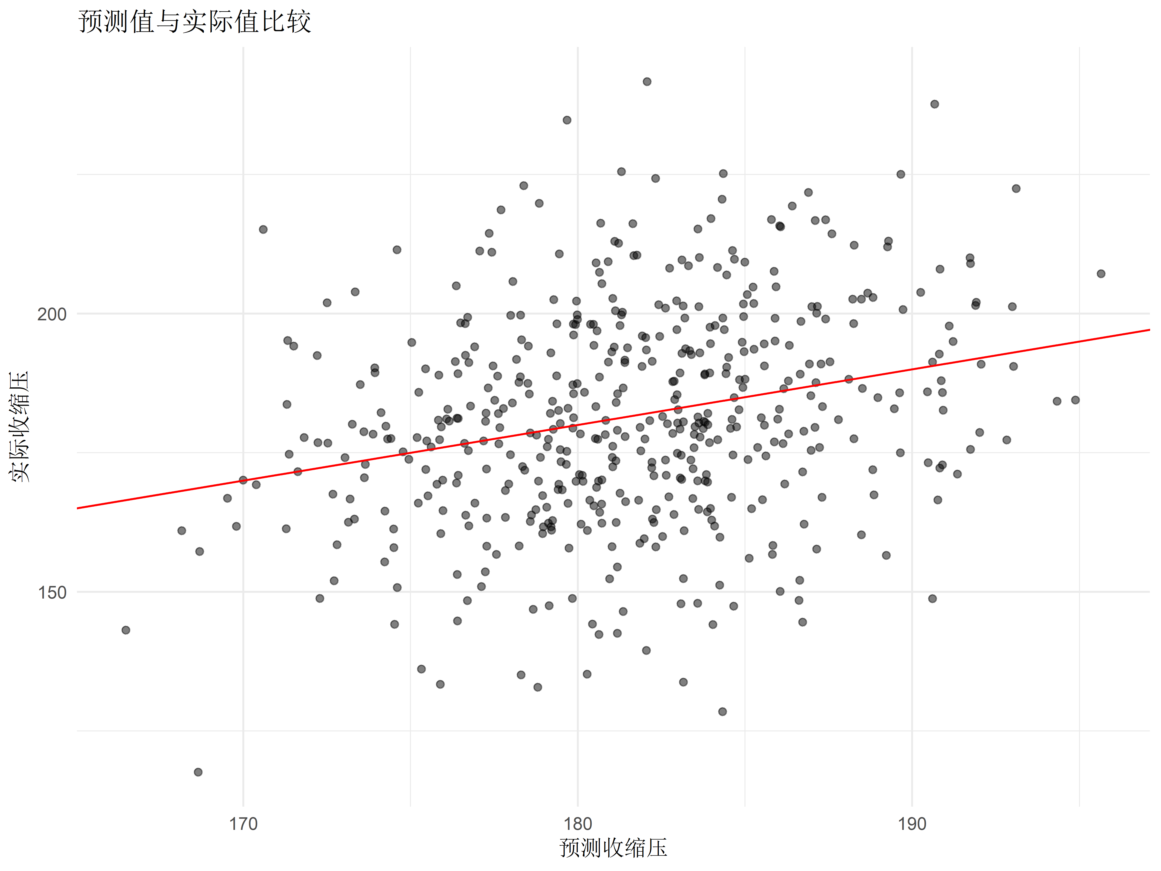
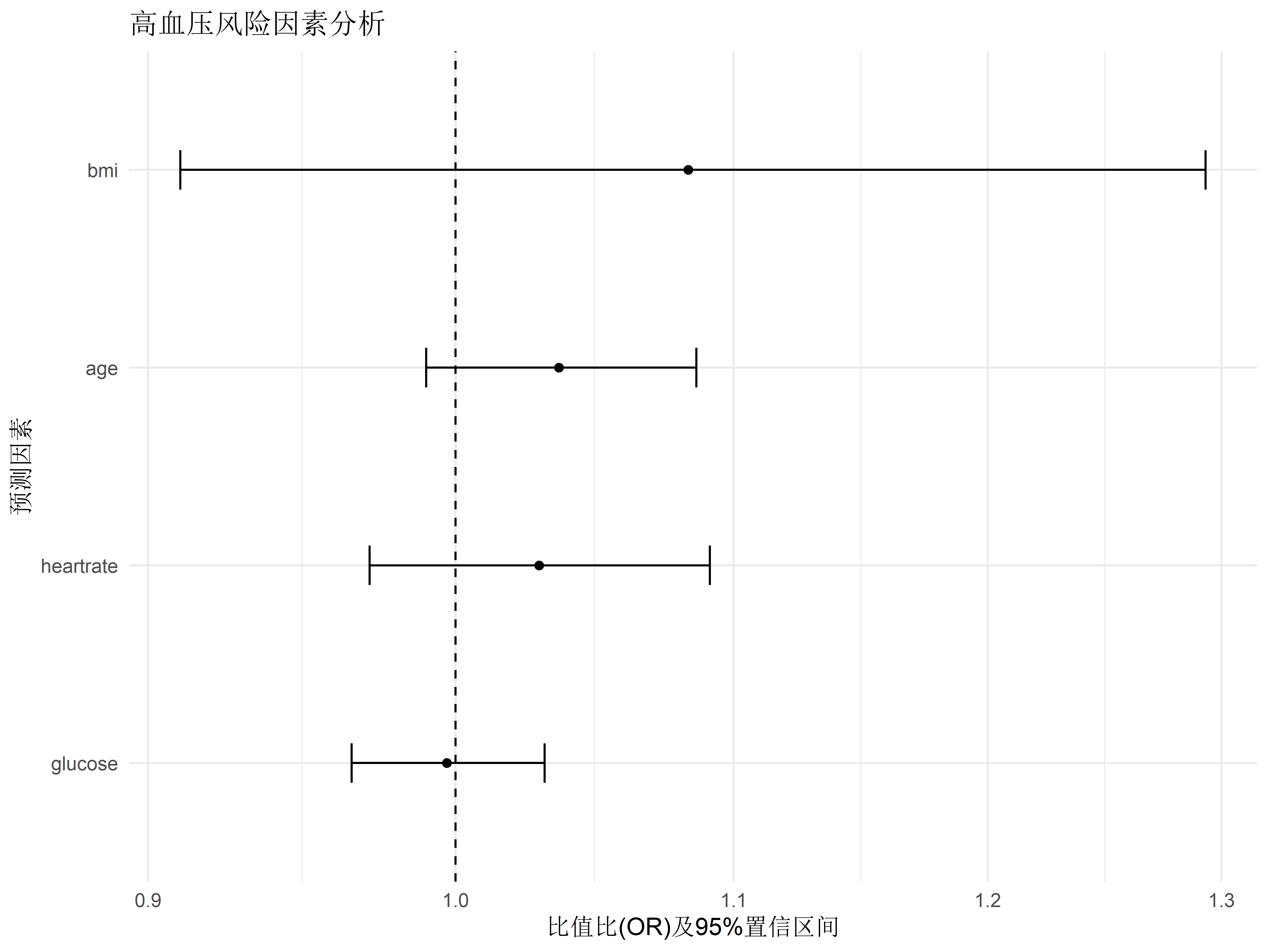
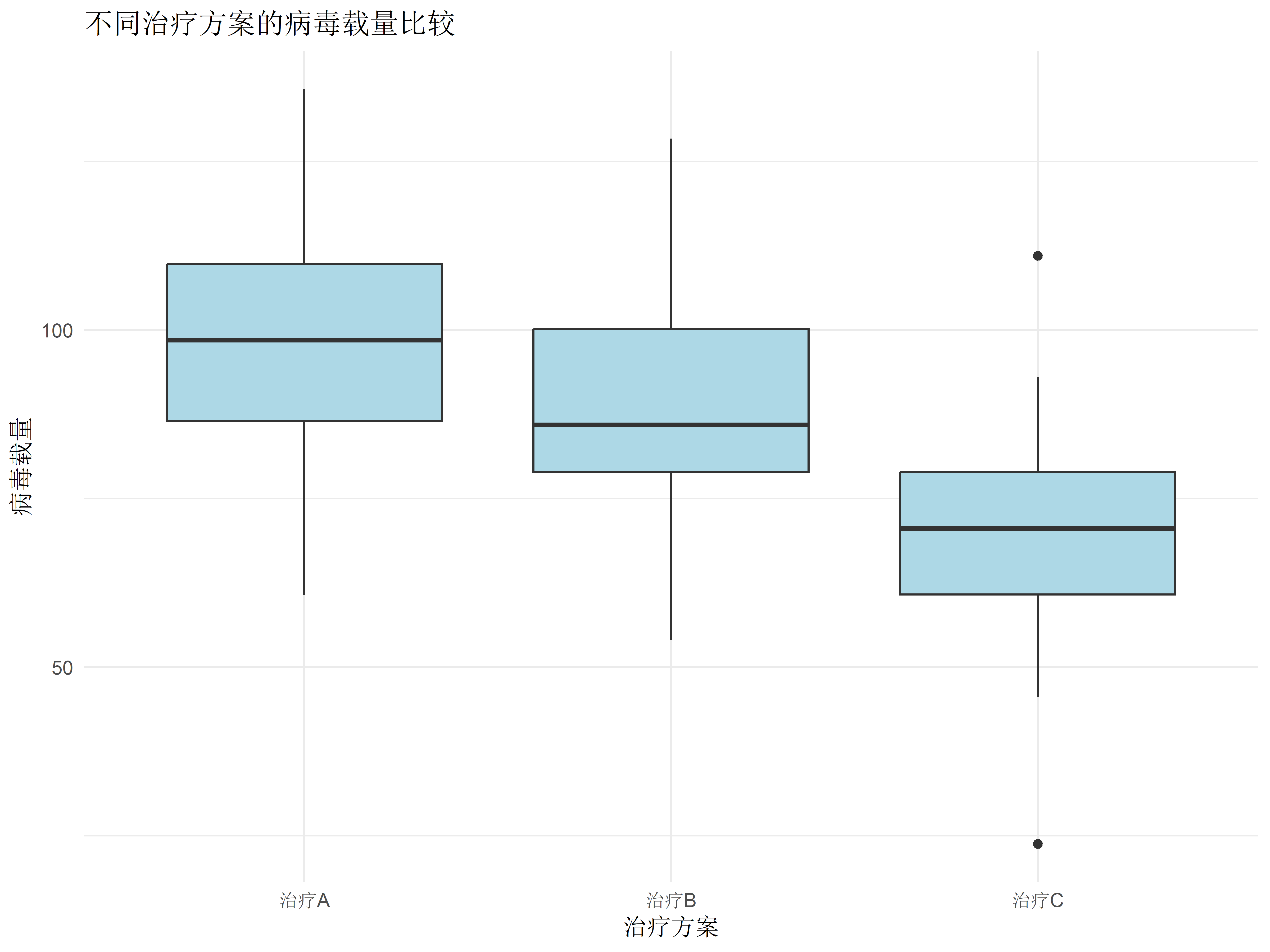
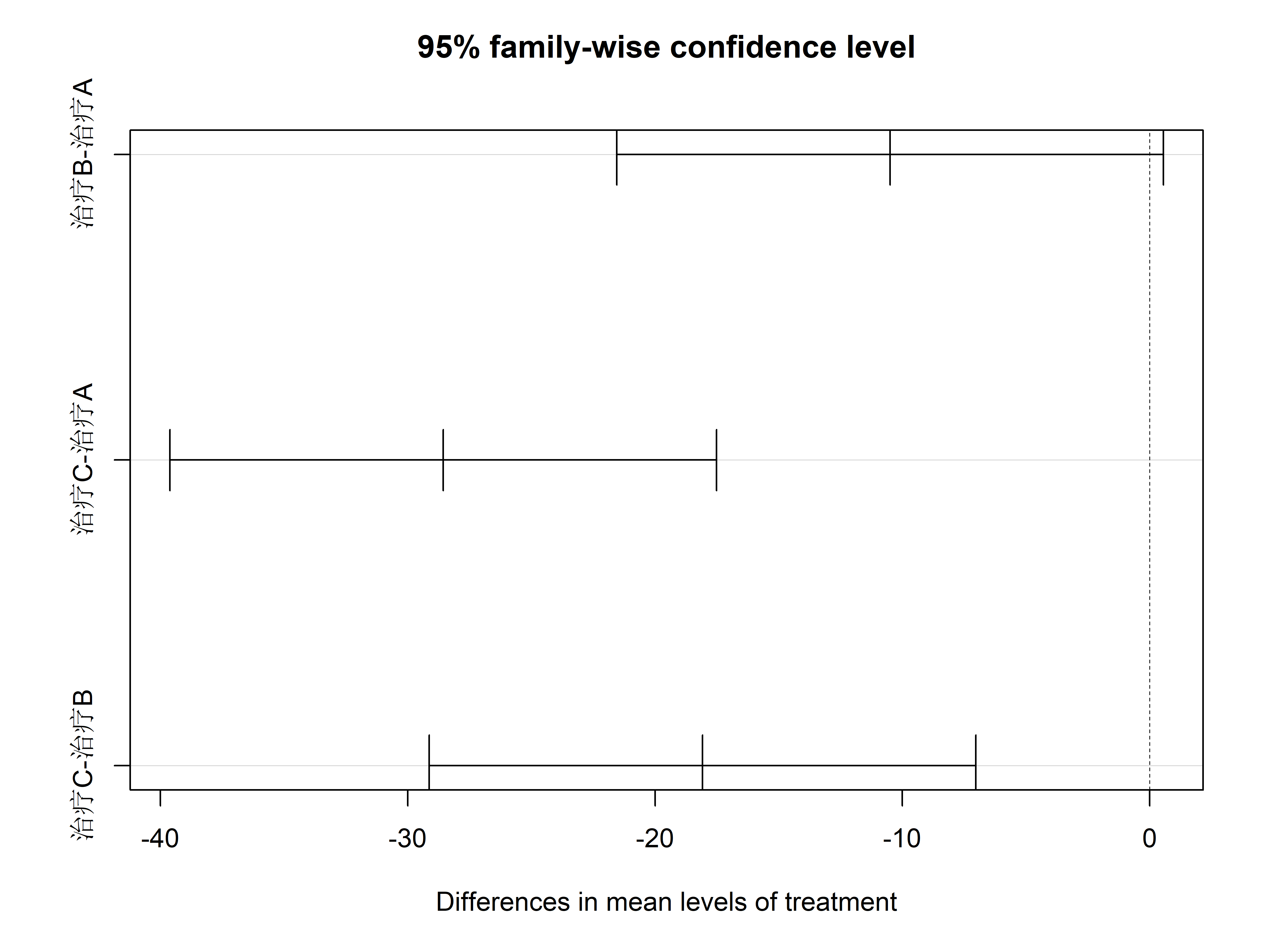
# 统计建模基础 {#sec-modeling-basics} ## 实践资源 ```{r} #| label: check-packages #| message: false # 设置CRAN镜像为中国合肥镜像 options (repos = c (CRAN = "https://mirrors.ustc.edu.cn/CRAN/" ))# 检查并安装所需的R包 <- c ("tidyverse" , # 数据处理和可视化 "broom" , # 模型结果整理 "car" , # 回归诊断 "medicaldata" , # 医学数据集 "TH.data" , # 示例数据 "survival" # 生存分析 # 检查并安装缺失的包 <- required_packages[! (required_packages %in% installed.packages ()[,"Package" ])]if (length (new_packages)) install.packages (new_packages, dependencies = TRUE )# 加载所有包 invisible (lapply (required_packages, library, character.only = TRUE ))``` ## 线性回归模型 {#sec-linear-regression} ### 血压影响因素建模 {#sec-bp-model} ```{r} #| label: setup #| message: false library (tidyverse)library (broom)library (car)# 创建模拟数据 set.seed (123 )<- 500 # 先创建基础变量 <- data.frame (age = rnorm (n, mean = 50 , sd = 15 ),bmi = rnorm (n, mean = 25 , sd = 4 ),heartrate = rnorm (n, mean = 75 , sd = 12 ),glucose = rnorm (n, mean = 100 , sd = 20 )# 然后添加依赖变量 $ sbp <- with (clinical_data, rnorm (n, mean = 130 , sd = 20 ) + 0.3 * age + 0.5 * bmi + 0.2 * heartrate + 0.1 * glucose# 构建多元线性回归模型 <- lm (sbp ~ age + bmi + heartrate + glucose, data = clinical_data)# 查看模型摘要 summary (bp_model)# 使用broom整理结果 <- tidy (bp_model, conf.int = TRUE ) %>% mutate (across (where (is.numeric), round, 3 ))# 可视化系数估计 ggplot (tidy_results, aes (x = reorder (term, estimate), y = estimate)) + geom_point () + geom_errorbar (aes (ymin = conf.low, ymax = conf.high), width = 0.2 ) + coord_flip () + labs (title = "收缩压影响因素分析" ,x = "预测变量" ,y = "回归系数估计值" ) + theme_minimal ()``` ### 模型诊断与验证 {#sec-model-diagnostics} ```{r} #| label: diagnostics # 模型诊断图 par (mfrow = c (2 , 2 ))plot (bp_model)# 多重共线性检验 vif (bp_model)# 预测值与实际值比较 <- augment (bp_model)ggplot (predictions, aes (x = .fitted, y = sbp)) + geom_point (alpha = 0.5 ) + geom_abline (intercept = 0 , slope = 1 , color = "red" ) + labs (title = "预测值与实际值比较" ,x = "预测收缩压" ,y = "实际收缩压" ) + theme_minimal ()``` ## 逻辑回归应用 {#sec-logistic-regression} ### 疾病风险预测模型 {#sec-risk-prediction} ```{r} #| label: logistic-model # 创建二分类结局 $ hypertension <- ifelse (clinical_data$ sbp >= 140 , 1 , 0 )# 构建逻辑回归模型 <- glm (hypertension ~ age + bmi + glucose + heartrate,family = binomial (link = "logit" ),data = clinical_data)# 模型摘要 summary (logit_model)# 计算OR值及置信区间 <- tidy (logit_model, conf.int = TRUE , exponentiate = TRUE ) %>% mutate (across (where (is.numeric), round, 3 ))``` ### OR值解读与报告 {#sec-or-interpretation} ```{r} #| label: or-plot # 创建森林图展示OR值 ggplot (or_results[- 1 ,], aes (x = reorder (term, estimate), y = estimate)) + geom_point () + geom_errorbar (aes (ymin = conf.low, ymax = conf.high), width = 0.2 ) + geom_hline (yintercept = 1 , linetype = "dashed" ) + coord_flip () + scale_y_log10 () + labs (title = "高血压风险因素分析" ,x = "预测因素" ,y = "比值比(OR)及95%置信区间" ) + theme_minimal ()``` ## 方差分析 {#sec-anova} ### 多组治疗方案比较 {#sec-treatment-comparison} ```{r} #| label: anova-analysis # 创建模拟治疗数据 set.seed (123 )<- 30 <- data.frame (treatment = factor (rep (c ("治疗A" , "治疗B" , "治疗C" ), each = n_per_group)),viral_load = c (rnorm (n_per_group, mean = 100 , sd = 20 ), # 治疗A组 rnorm (n_per_group, mean = 85 , sd = 20 ), # 治疗B组 rnorm (n_per_group, mean = 70 , sd = 20 ) # 治疗C组 # 进行单因素方差分析 <- aov (viral_load ~ treatment, data = treatment_data)summary (aov_result)# 可视化组间差异 ggplot (treatment_data, aes (x = treatment, y = viral_load)) + geom_boxplot (fill = "lightblue" ) + labs (title = "不同治疗方案的病毒载量比较" ,x = "治疗方案" ,y = "病毒载量" ) + theme_minimal ()``` ### 事后检验(Tukey HSD) {#sec-post-hoc} ```{r} #| label: tukey-test # Tukey事后检验 <- TukeyHSD (aov_result)print (tukey_result)# 可视化事后检验结果 plot (tukey_result)``` ## 练习 1. 使用自己的数据构建线性回归模型2. 进行完整的模型诊断3. 构建疾病预测模型并评估其性能4. 比较多个治疗组的效果## 本章小结 1. 线性回归模型的构建和诊断2. 逻辑回归在疾病预测中的应用3. 方差分析的实施和解释4. 如何正确报告统计结果